![]()
Translating Machine Learning Outputs Using Shapley Values

![]()
One thing is guaranteed for every data scientist: when you face the problem of classification or regression, you always have to complete a series of actions crucial to the quality of the final output. These actions can be broken down into three steps.
And while a data scientist may have control over training, generally regarding data selection, they’re still often challenged with empowering people who aren’t tech-savvy to benefit from artificial intelligence-based results.
For example, a data scientist may need to explain to a physician — who typically has little experience with mathematics and statistics — the reasons an AI-based mechanism predicted whether a patient is at risk of suffering from a heart attack. This information is crucial for many reasons: from a health point of view, the usability of such information can allow the physician to provide the best treatment to each single patient, as well as to focus on more at-risk patients; from a technical point of view, the physician can better understand the combination of features that provided a particular output.
So a data scientist’s common challenge is explaining a model’s output — in this case, predictions regarding a patient — not just to people who aren’t familiar with mathematics and statistical modeling, but to themself to better understand which features have a bigger impact on the model’s outcome.
Indeed, most of the time a model’s output is used differently by different stakeholders, who have varying needs as well as varying technical and analytical skills. What we, as machine learning specialists, think of as simple (such as a querying a DWH to get information about a particular user or interpret a probability measure), is, for many, incredibly confusing.
That’s why a data scientist often finds themself between the so-called inference accuracy and the explainability dilemma. Nowadays, excellent production performance isn’t enough; one must be able to democratize the result, allowing a potentially heterogeneous and fragmented audience of people to understand the final result.
Recently, the concept of eXplainable AI (XAI) has become popular and a few solutions have been proposed in order to make black-box machine learning models not only highly accurate, but also highly interpretable by humans. Among the emerging techniques, two frameworks have been widely recognized as the state-of-the-art: the Lime framework and the Shapley values.
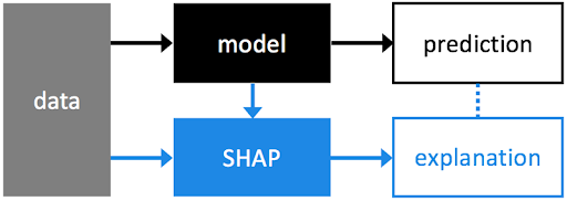
The goal of this blog post is essentially to shed light on the use of Shapley values in order to easily explain the result of any Machine Learning model, and to make the output available to a greater audience of stakeholders. In particular, we will use the python SHAP (SHapley Additive exPlanations) library, which was born as a companion of this paper and which has become a point of reference in the data science field. For more details, we invite you to look at the online documentation, which contains several examples from which you can get inspired.
Here at Cloud Academy, we had a Webinar series entitled Mastering Machine Learning, where we discussed – in more general terms – the use of the SHAP library with respect to a Classification task. You can find a detailed description of the agenda here.
Let’s talk about a famous dataset: the Wine Quality Dataset. It consists of a catalog of white and red wines, related to the Portuguese variant Vinho Verde, containing useful information for describing and evaluating the wine itself. For the sake of this example, we’ll only use the red wine dataset with the goal of classifying the quality of each single example.
To support this analysis, you can find a notebook here, where the entire data processing and fitting pipeline is illustrated. Assuming we selected the best classifier, we may encounter a possible dilemma that we can summarize as follows. Two examples, illustrated below:
| fixed acidity | 7.0000 | fixed acidity | 8.0000 |
| volatile acidity | 0.60000 | volatile acidity | 0.31000 |
| citric acid | 0.30000 | citric acid | 0.45000 |
| residual sugar | 4.50000 | residual sugar | 2.10000 |
| chlorides | 0.06800 | chlorides | 0.21600 |
| free sulfur dioxide | 20.00000 | free sulfur dioxide | 5.00000 |
| total sulfur dioxide | 110.00000 | total sulfur dioxide | 16.00000 |
| density | 0.99914 | density | 0.99358 |
| pH | 3.30000 | pH | 3.15000 |
| sulphates | 1.17000 | sulphates | 0.81000 |
| alcohol | 10.20000 | alcohol | 12.50000 |
These two wines look very similar, but they’re technically different. In practice, our model — which is, in this case, an XGBoost model (Extreme Gradient Boosting) — can learn very detailed patterns in the data that may not be super obvious to the data scientist working the dataset.
In the example in Figure 2, the model correctly predicts the class of bad wines (Figure 2, left) and the class of high-quality wines (Figure 2, right). The performance of the machine learning model is, therefore, good, but we’re left with the task of explaining results in a convincing way. Which features positively affect the output score? Is there any way to see the contribution, in terms of probability score, of each single feature in the final output?
In their seminal paper, Lundeberg and Lee (2017) used a famous idea from American Nobel Price-winning economist and mathematician Lloyd Stowell Shapely to propose an idea describing the output score of a machine learning model. This idea uses his Nobel prize contribution, known as the Shapley value solution in cooperative game theory, to describe the impact of each single feature to the final output score.
More specifically, the Shapley value is based on the idea that the payoff obtained from a particular cooperative game should be divided among all participants in such a way that each participant’s gain is proportional to their contribution to the final output. This makes sense; everyone contributes differently to the output. This characteristic is particularly useful in machine learning, since we want to divide the overall probability score based on how much each single feature has contributed to it.
The SHAP (Python) library is a popular reference in the data science field for many reasons, especially because it provides several algorithms to estimate Shapley values. It provides an efficient algorithm for tree ensemble models and deep learning models. But, more importantly, SHAP provides a model-agnostic algorithm used to estimate Shapley values for any kind of model. An exciting development: recently, a model compatible with Transformers for NLP tasks was made available in the library.
So why is this library useful? Well, we have at least two major explanations that can be simplified with two simple concepts: Global and Local interpretability.
We’ll begin by framing the problem with a more practical argument. Consider the concept of simple arithmetic mean, e.g., what was your average grade at university? If this sounds familiar to you, then you know the average gives you a general idea of the (physical) patterns — like a general idea of how you performed at university.
However, the mean has a huge problem: it is sensible to outliers, but it completely loses the interpretability of local behaviors. What does that mean? Well, an average grade doesn’t tell you how you performed on a particular topic on a particular exam.
The idea of the Shapley values is to go beyond the simple concept of mean, since the values explain a model’s output with respect to all observations (Global interpretability) and each single observation (Local interpretability) because they build a quantitative indicator based on the feature’s values.
Let’s dive into the concept of Global interpretability. Consider a Random Forest Classifier, or any Gradient Boosting-based Classifier, like XGBoost. Training such models means making decisions based on feature values. Technically speaking, the impact of each single feature has on the tree’s splits can be tracked using metrics, which is typically identified by the Mean Decrease Impurity (MDI) criterion.
From a historical point of view, the MDI is also called Gini Importance — named in honor of the Italian Statistician and Economist Corrado Gini, who developed the Gini index, a measure of the income inequality in a society — and used as the splitting criterion in classification trees.
The idea behind this criterion is pretty straightforward: every time a split of a node is made on a specific variable, the Gini impurity criterion for the two descendent nodes is lower than the parent node. The Gini Importance computes each feature importance as the sum over the number of splits — across all trees — that include the feature proportional to the number of samples it splits.
This is, more generally, called Global Feature Importance (or Global Interpretability) because it takes into account several interactions of the same features across different trees. Put in simpler terms, we can say that the global importance is nothing more than an average over all samples for the contribution of that particular feature during the splitting phase of the tree across all trees. This has a major limitation: it completely loses the explanation for individual observations.
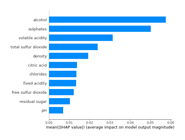
We can, instead, build a global feature importance based on the Shapley values we observed for each single feature. Then, the SHAP global feature importance is computed using the shapley magnitude of feature attributions. For each single feature, we compute the mean absolute value of the corresponding shapley value for each single observed statistical unit. In this way, we can generalize local contributions to the overall population. In Figure 3, you’ll find an example of Global Importance based on the mean SHAP value.
Shapley values can go beyond the classical global feature importance. Thanks to the estimated Shapley values, we can compute the impact of each single feature on the model prediction for any machine learning model. This is the core of local interpretability, since we can explain each single predicted outcome based on the feature’s values. Indeed, the Shapley values computed for a specific wine allows us to describe the impact of each single feature with respect to the model outcome.
But how does it work?
From a technical point of view, we can identify two important aspects:
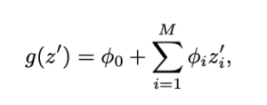
where phi describes the Shapley value for each single feature, denoted by z, and phi_0 denotes the base value. Each single phi value is calculated by taking into account all possible values computed on the considered feature for all possible combinations of features. Check out section 2.4 of the original paper for more details.
Also, note that the Shapley values should be estimated from a model. In this notebook, we’ve fitted an XGBoost Classifier, being the state-of-the-art for these types of prediction problems with tabular style input data of many modalities (typically, numerical and categorical features). We used a TreeExplainer as the underlying SHAP model to explain the output of our ensemble tree models. If you’re interested in learning more, do read the original paper. There are many other SHAP explainers, such as the
From a performance point of view, it’s recommended that you the TreeExplainer with any ensemble tree model (e.g. scikit-learn, XGBoost, catboost). It is, however, possible to use a KernelExplainer, though SHAP model performances might get worse with large batches of data.
For the sake of illustration, let’s consider the following figure that shows the impact of each single feature on the model prediction.

In particular, the blue segments describe the impact of the features that contribute the most to increase the prediction score, whereas the red ones are the factors that reduce the impact. This kind of visualization of the model’s outputs is a great tool that allows everybody to understand which features have had the greatest impact on the final model score.
In summary, we learned how to employ the Shapley value to explain any machine learning model output. We used the SHAP python library, which comes with many models and features that easily help the Data Scientist to convert a technical result into a friendly, human-interpretable explanation.