![]()
Azure Machine Learning: A Cloud-based Predictive Analytics Service
Last week I wrote about using AWS’s Machine Learning tool to build your models from an open dataset. Since then, feeling I needed more control over what happens under the hood – in particular as far as which kind of models are trained and evaluated – I decided to give Microsoft’s Azure Machine Learning a try.
In case you’re not yet familiar with Microsoft Azure, we are talking about a Platform as a Service (PaaS) and Infrastructure as a Service (IaaS) solution created by Microsoft back in 2010. Cloud Academy has some excellent courses introducing you to the platform.
Azure Machine Learning was launched in February this year, and was immediately recognized as a game changer in applying the power of the cloud to solve the problem of big data processing.
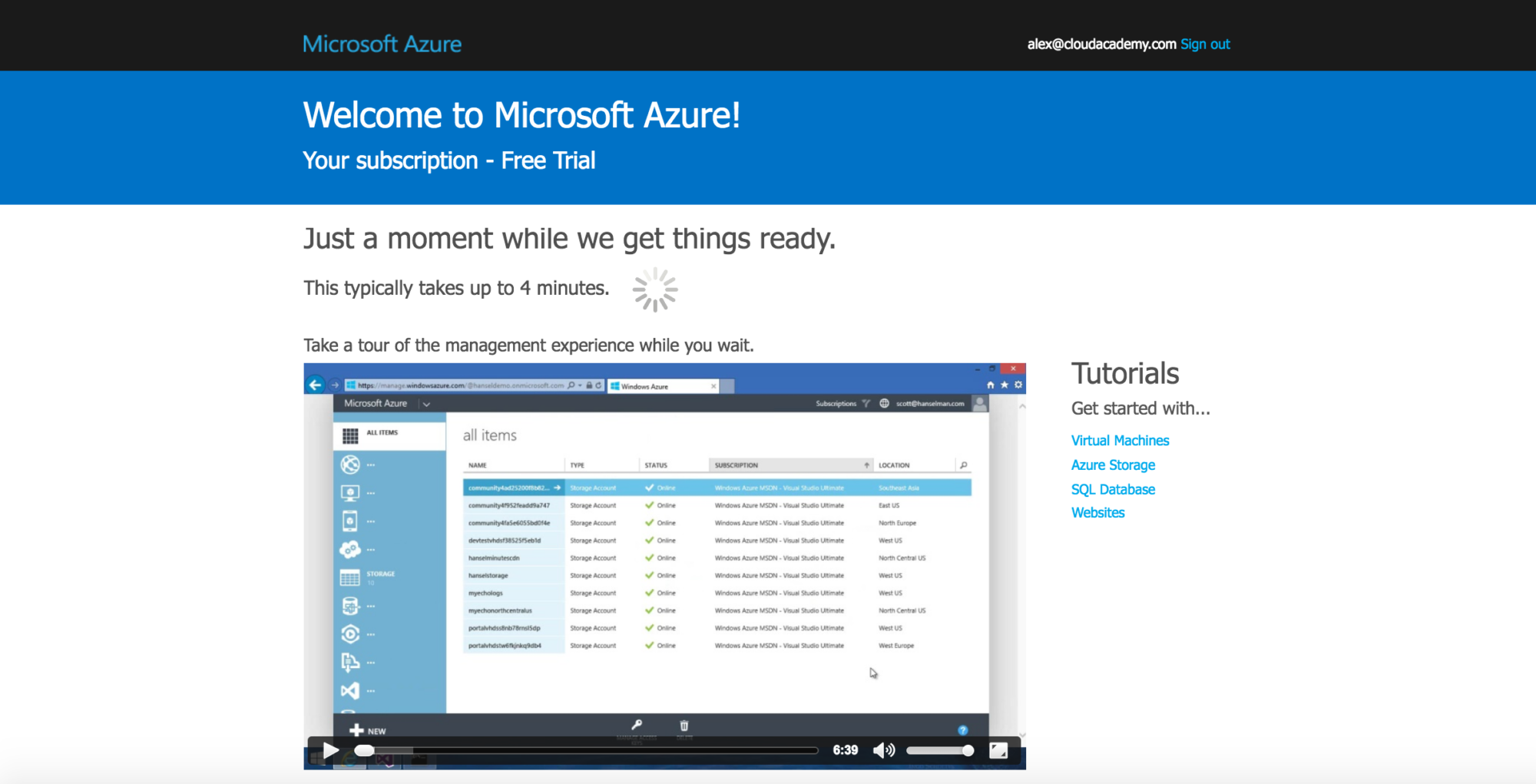
Since I’m new to the Azure world, I decided to start my 1 month free trial (including $150 of credit). My dashboard was up and running within a few minutes, during which I gladly took a quick tour of the dashboard features.
After just a few clicks I discovered that Azure Machine Learning offers a fairly independent environment to work on. To be precise, it’s called ML Workspace and is where all your ML-related objects live, although we will still be able to monitor our ML web services directly from the general Azure dashboard.
First step: create an Azure Machine Learning Workspace
This was quite simple: every time you want to create something you’ll find a “+ New” button on the bottom left part of your dashboard. Here I looked for “Machine Learning” in the “Data Services” section. The creation process is straightforward: provide names for the Workspace and for the new storage account.

You can always access your Azure Machine Learning Studio, which is where I spent most of my time. The workspace UI is coherent and clear, although the dependency between items might not always be immediately evident. Let’s briefly describe what kind of items you’re going to work on.
- Datasets. As you would image, these are our data containers. You can only create a new one from a local file, although there are other ways to feed our models via special Reader objects.
- Experiments. An experiment is a set of connected components used to create, train, score, and test our model. Additional modules can be added to take care of data preprocessing, features selection, data splitting, cross-validation, etc. You can find plenty of them to import here.
- Trained Models. Once you are happy with the model on which you’ve experimented, you can save it and even reuse it in future experiments.
- Web Services. In order to obtain new predictions (either online or batch predictions) we’ll need to create and query a Web Service. Azure will even help by creating documentation and sample code for accessing its endpoints (via simple POST requests).
How to import your dataset
As with my previous article about Amazon Machine Learning, I will be using an open dataset, specifically designed for Human Activity Recognition (HAR). It contains 10,000 records, each defined by 560 features (input columns), plus one target column that represents the activity type we want to classify. The authors have manually labeled each row with one of six possible activity types, which means we are trying to solve a multiclass problem.
Once again, we’ll be manipulating the raw dataset to create one single csv file (see this Python script), although we could also have used one of these formats as input for our Dataset object:
- CSV (with or without header row)
- TSV (without or without header row)
- Plain Text (.txt)
- ZIP (.zip)
- SvmLight (more info here)
- ARFF (Attribute Relation File Format)
- RData (R Object or Workspace)
But those aren’t the only ways to bring data into Azure Machine Learning. We might use a special Reader object in our experiments to retrieve data via one of the following:
- Web URL (HTTP)
- Azure Blob Storage
- Azure SQL Database
- Azure Table
- Hive Query
- Data Feed Provider (Odata)
OK, let’s import our csv file (without a header row) and create a new Dataset object. This step might take a while, based on your network speed, but you can continue working on your experiment.
How to create an Azure Machine Learning model
Unexpectedly, working on Experiments is quite fun. As soon as you create your first blank experiment, you’re shown a very user-friendly UI with a lot of building blocks to link together in order to train and evaluate your model.
You have full control over what’s going on and each input and processing phase can be configured or removed at any time.

First things first: I dragged in my Dataset object (I named it “HAR dataset (csv)”, as you can see in the screenshot above) and, of course, not much happened. This is when I had to decide which model to use.
You can find all the available models in the “Machine Learning > Initialize model” menu on your left. Here I selected “Classification” and focused on the Multiclass models (Decision Forest, Decision Jungle, Logistic Regression, and Neural Network).
For the purpose of this demonstration, let’s assume I directly chose “Logistic Regression” although, in truth, I came to this conclusion only after training and evaluating both Logistic Regression and Neural Network (which I will show how at the end of this article).

Note: when you drag the “Logistic Regression” block into your experiments, in practice you are only creating a model configuration object. It will contain all your model parameters, which you can always edit, even after running an experiment.
In order to actually train a model, a “Train Model” object is needed. You can find it in the “Machine Learning > Train” menu.

Each block can be connected to a set of inputs and outputs (the experiment won’t even run if every required connection is not filled). Our Train Model block takes as input an Untrained Model (our model config) and a Dataset object. The UI will really help you, as you can see the input/output type by simply hovering your mouse on the connection slot.
We’re not yet done with training. We still need to let our new block know which is the target column we’re trying to predict.
On the Train Model properties sidebar, I can click on “Launch column selected” or choose the “Col1” variable as target column. Note that, since we uploaded a header-less csv file, our columns are not named, but automatically receive an incremental number.
But it’s not going to be quite so simple. We want to create a model and then be able to understand how it performs. A general solution is splitting your dataset into two random sets (let’s say 70/30), using 70% of your dataset to train a robust model, and then testing it against the remaining 30%. This is to ensure that your model behaves well with new data.
Not a big deal. We can just add a new “Split” block. It takes only one input (our Dataset object) and gives you two output links, based on the “Fraction of rows” parameter. You can try to tune it across several experiments runs and see what changes (maybe 60/40? or 50/50?).

Now, what can we do with our “Train Model” block output? It is, in fact, a trained model, so we’ll put it to work. We add a “Score Model” block to verify that it can take the remaining 30% of our dataset and generate actual predictions.
Once everything is configured, we can finally run our experiment (yes, by clicking the big “Run” button at the bottom!). Incredibly, it takes just a few seconds (about ten seconds with this dataset). Now you can quickly inspect the results by clicking on the output of our new “Score Model” block, and then on “Visualize”.

Here we can find the predicted class for each of our 3,090 rows, together with statistics about each column, including mean, median, min, max, standard deviation, and a graphical distribution of its values (histogram).
Of course, manually reading through 3,000 rows is not how we evaluate our model: we’ll need to add one last “Evaluate Model” block (“Machine Learning > Evaluate” menu).
We’ll quickly re-run the experiment, click on the evaluation block output, and then “Visualize”.
Here we find very useful data about our model accuracy, precision, and recall. More intuitively, you can graphically visualize how the 6 possible classes have been classified in the testing set by looking at the Confusion Matrix. I got pretty good results using Logistic Regression, ranging from 94% to 100% precision. You may also notice particular patterns, for example, those “squares” around the classes 1, 2, 3 and 4 and 5. This happens when classes are, indeed, confused by your model. In our case 1, 2, and 3 are the “walking” classes, while 4 and 5 are “sitting” and “standing”. We expected to have some problems with their predictions the way we had with Amazon Machine Learning. With Amazon Machine Learning, however, we achieved a 100% precision for the “laying down” activity!

How to use the model in your code
In order to finally use our model for real-time predictions, we need to expose it as a Web Service. In fact, Web Services can be created for the result of an experiment inside Azure Machine Learning. Luckily, converting the already created experiment to your first Web Service is fairly painless, requiring only a click on “Create Scoring Experiment”. You can also enjoy a beautiful animation by watching this video if you just can’t wait for your own.
One thing I didn’t notice at first is that every experiment has a “Web Service switch”. Eventually, you can define your training/testing procedure and your web service within the same experiment, switching back and forth between the two visualizations (they simply highlight/blur some input/output blocks).
We’re almost there. There’s just one more task before publishing our web service: we need to name “Web Service Input” and “Web Service Output” blocks. I named mine “record” and “result.” These names will be used as JSON fields in the web service response.
We can finally run the experiment one last time and click on “Publish Web Service”.

Azure Machine Learning automatically creates an ad-hoc API key and a default endpoint for your published web service. That really is all you’ll need. At the very bottom of your web service’s public documentation page, you’ll find sample code for C#, Python, and R.
Here is the simple Python script I coded based on the default one:
import urllib2
import json
#web service config
webservice = 'YOUR_WS_URL'
api_key = 'YOUR_WS_KEY'
#dataset config
labels = {
	'1': 'walking', '2': 'walking upstairs', '3': 'walking downstairs',
	'4': 'sitting', '5': 'standing', '6': 'laying'
}
n_classes = len(labels)
n_columns = 562
#read new record from file
with open('record.csv') as f:
	record_str = f.readline()
#POST data
input_data =  {
    "Inputs": {
        "record":{
        	"ColumnNames": ["Col%s" % n for n in range(1,n_columns+1)], #dynamic
            "Values": [ ['0'] + record_str.split(',') ] #leading zero
        },
    },
    "GlobalParameters": {}
}
#request config
headers = {'Content-Type':'application/json', 'Authorization':('Bearer '+api_key)}
req = urllib2.Request(webservice, json.dumps(input_data), headers)
try:
    data = json.loads(urllib2.urlopen(req).read())
    result = data['Results']['result']['value']['Values'][0] #too deep?
    label = result[-1] #last item is our classified class
    stats = result[-(n_classes+1):-1] # M probabilities, one for each class
    print("You are currently %s. (class %s)" % (labels[label], label) )
    for i,p in enumerate(stats):
    	print("Scored Probabilities for Class %s : %s" % (i+1, p))
except urllib2.HTTPError as e:
    print("The request failed with status code: " + str(e.code))
    print(e.info())
    print(json.loads(e.read()))
I did notice that Azure Machine Learning causes a lot of data to travel a great deal across the network. The POST request is pretty heavy of course since we are sending more than 500 input values (with their auto-generated variable name).
What surprised me is how unnecessarily heavy their response format – a JSON table – is, since it contains the input record we’ve just sent, together with the predicted class and all the other classes’ reliability measure. Indeed, in our case, it contains about 18KB of data and the HTTPS call takes about seven seconds (versus the two seconds we experienced with Amazon Machine Learning).
UPDATE: as our reader, Dmitry clarified with his comment below, we can easily reduce the size of every response by placing a “Project Columns” module right before the “Web Service Output” one.
This way – projecting only “all scores” and “all labels” – I managed to cut the response size down to only 560B, although the response time is still about 7 seconds.
{
    "Results": {
        "result": {
            "type": "table",
            "value": {
                "ColumnNames": [
                    "Col1",
                    "Scored Probabilities for Class \"1\"",
                    "Scored Probabilities for Class \"2\"",
                    "Scored Probabilities for Class \"3\"",
                    "Scored Probabilities for Class \"4\"",
                    "Scored Probabilities for Class \"5\"",
                    "Scored Probabilities for Class \"6\"",
                    "Scored Labels"
                ],
                "ColumnTypes": [
                    "Numeric",
                    "Numeric",
                    "Numeric",
                    "Numeric",
                    "Numeric",
                    "Numeric",
                    "Numeric",
                    "Categorical"
                ],
                "Values": [
                    [
                        "0",
                        "0.00638132821768522",
                        "0.970375716686249",
                        "0.0132338870316744",
                        "0.000609736598562449",
                        "0.00881590507924557",
                        "0.000583554618060589",
                        "2"
                    ]
                ]
            }
        }
    }
}
Anyway, what we’re after is the “Scored Labels” column (the very last one!). It contains an integer that represents the predicted class for the given record.
Furthermore, the M previous columns contain “Scored Probabilities for Class N”: as already mentioned for AWS ML, these values might help you take more advanced decisions in case the selected prediction by your model is not reliable enough.
Note: there exists an Azure SDK for Python – and even a read-only Azure Machine Learning client – but it can’t be used to access your Web Service. I can see how my new web service is not particularly hard to query, but honestly, I would rather access it with a well structured and tested client than using raw http(s) requests and JSON parsing.
Monitoring your Web Service
If your model works fine and you (and your team) have access to its endpoint and API key, your web service will start serving predictions on new data. You may want to monitor its load.
You can find all your Azure Machine Learning web services on the general Azure dashboard, inside the “Web Services” section of your Azure Machine Learning Workspace.
Here you can find a detailed visualization of all the requests (predictions), for each configured endpoint.
 Furthermore, you can create new endpoints and configure their Throttle level and Diagnostics Trace level. Of course, this can be used to monitor separately or to grant/remove temporary access to your Web Service. Note that you can’t delete your default endpoint. For example, I have created a “dev” endpoint with a “Low” Throttle level and “All” Diagnostics Trace level, to be used for development, so it won’t be confused with production loads and statistics.
Experiments with many models
As promised, I’m going to discuss how to create an experiment to train and test more than one model at once.
Basically, you just have to add more parallel blocks to your diagram and use the output of your first blocks multiple times. Once you have configured and scored two different models, you can reuse the Evaluate Model block, which can take an additional Scored Dataset object as input.
Let’s see how I trained and evaluated both Logistic Regression and Neural Network models with the very same dataset.

… and much more
While my goal was to reproduce the same ML model I created on AWS last week, I’ve found out that Azure Machine Learning is much more than just Machine Learning as a Service. You can, in practice, create any data science workflow, using a ready-to-use set of modules to manipulate and analyze your data, including:
- Data conversion and transformation.
- Feature Selection (Filter-based, Fisher LDA, etc).
- OpenCV algorithms (Image Reader and Cascade Image Classification).
- Python scripts (the script must contain an azureml_main function and eventually import zipped libraries).
- R models and scripts.
- Statistical Functions (correlation, trigonometric transformations, rounding, deviation, kurtosis, etc).
- Text Analytics (Feature Hashing, Named Entity Recognition, etc).
Once again, you can learn how to use all these amazing tools by exploring the Azure Machine Learning Gallery. You can even add your own experiments to the list.
If you want to get learn more on Azure Machine Learning, this is your go-to learning path: Introduction to Azure Machine Learning.